graph TB
    subgraph Space["Sample Space (Ω)"]
        direction LR
        O1["ω₁"]
        O2["ω₂"]
        O3["..."]
        On["ωₙ"]
        SpaceCaption["All possible outcomes<br/>from our random experiment"]
        O1 & O2 & O3 & On --- SpaceCaption
    end

    subgraph Range["Range of X"]
        direction LR
        X1["x₁"]
        X2["x₂"]
        X3["..."]
        Xm["xₘ"]
        RangeCaption["Numerical values<br/>X: Ω → ℝ"]
        X1 & X2 & X3 & Xm --- RangeCaption
    end

    %% Connections with labels
    O1 -->|"X"| X1
    O2 -->|"X"| X2
    O3 -->|"X"| X2
    On -->|"X"| Xm

    %% Styling
    classDef default fill:#f8f8f8,stroke:none,color:#000
    classDef outcomes fill:#e1f5fe,stroke:#333,stroke-width:2px,color:#000
    classDef values fill:#e8f5e9,stroke:#333,stroke-width:2px,color:#000
    classDef caption fill:none,stroke:none,color:#000

    class O1,O2,O3,On outcomes
    class X1,X2,X3,Xm values
    class SpaceCaption,RangeCaption caption
19 Random Variables and Probability Distributions
Understanding Random Variables and Probability Distributions: Mathematical Models for Randomness
Beyond Classical Probability
The classical approach to probability (calculating favorable outcomes divided by total possible outcomes) rests on a crucial assumption: we have perfect knowledge of how our outcomes are generated.
For instance, when we say a coin is fair, we assume its physical properties and flipping mechanism produce heads and tails with exactly equal probability.
But how do we know this? In real-world scenarios:
- Physical coins may be slightly unbalanced
- Flipping mechanisms might favor certain outcomes
- Environmental factors could influence results
- Manufacturing processes could introduce bias
This highlights a fundamental challenge: we often observe outcomes first and then must infer the underlying process that generated them. This is where random variables and probability distributions become essential tools:
- A Random Variable (RV) is a function that assigns a numerical value to each outcome in a sample space S:
- Allow us to model uncertain outcomes mathematically
- Bridge the gap between physical events and numerical analysis
- Enable quantitative description of patterns in observed data
- A Probability Distribution is a list of all of the possible outcomes of a random variable with their corresponding probabilities:
- Describe how likely different outcomes are
- Can be adjusted based on observed data
- Include classical probability as a special case
- Allow for modeling of biased or uneven processes
Think about flipping a coin 100 times and getting 47 heads. Is the coin fair? What’s the actual probability of heads?
To answer these questions rigorously, we need to:
- Model the underlying random process (data-generating mechanism)
- Connect our observations to this theoretical model
- Make precise statements about probabilities of different outcomes
Random Variables and Probability Distributions
A random variable X is a function that assigns a numerical value to each outcome in a sample space S. More formally, it’s a function X: S \rightarrow \mathbb{R} that maps outcomes from our sample space to real numbers.
For example: when flipping a coin, we might define X(H) = 1 for heads and X(T) = 0 for tails. This formalization helps us model the data-generating process.
For discrete random variables, the probability distribution is described by its Probability Mass Function (PMF) p_X(x) or P(X = x), which specifies our model’s assumptions about how likely each outcome is. A valid PMF must satisfy:
- Non-negativity: p_X(x) \geq 0 for all x
- Total probability: \sum_{x} p_X(x) = 1
For our (possibly unfair) coin: P(X = x) = p_X(x) = \begin{cases} p & \text{if } x = 1 \text{ (heads)} \\ 1-p & \text{if } x = 0 \text{ (tails)} \\ 0 & \text{otherwise} \end{cases}
where p is the true probability of heads that we’re trying to understand.
This framework lets us move beyond simply counting favorable outcomes to modeling and understanding the underlying random processes that generate our observations. It forms the foundation for working with more complex probability distributions and statistical inference.
Note: When dealing with continuous random variables (like height, weight, or time), we use Probability Density Functions (PDF) instead of PMFs. PDFs require calculus and integration to work with probabilities, which is beyond the scope of this course. We’ll focus exclusively on discrete random variables and their PMFs.
In summary, we need two key mathematical tools:
- A way to convert random outcomes into numbers (Random Variables)
- A way to describe how likely each number is (Probability Distributions)
Random Variable (RV): Making Randomness Measurable
A random variable (RV) is our bridge between unpredictable outcomes and their probabilities. It works in two steps:
- First, it maps outcomes to numbers
- Then, the probability distribution maps these numbers to their probabilities
A Random Variable is a function that converts unpredictable outcomes into numbers we can work with:
💡 Key Insight: RVs turn abstract outcomes into concrete numbers. For example:
- Converting “Heads/Tails” to “1/0”
- Counting successes in multiple trials
- Measuring waiting times
Probability Distribution Function (PDF): Describing Patterns of Randomness
Once we have numbers, we need to describe how likely each value is:
graph TB
    subgraph Values["Possible Values"]
        direction LR
        X1["x₁"]
        X2["x₂"]
        X3["..."]
        Xm["xₘ"]
        ValuesCaption["Numbers from our RV"]
        X1 & X2 & X3 & Xm --- ValuesCaption
    end

    subgraph Prob["Probabilities"]
        direction LR
        P1["f(x₁)"]
        P2["f(x₂)"]
        P3["..."]
        Pm["f(xₘ)"]
        ProbCaption["f: ℝ → [0,1]<br/>Must satisfy: Σf(xᵢ) = 1"]
        P1 & P2 & P3 & Pm --- ProbCaption
    end

    %% Connections
    X1 -->|"f"| P1
    X2 -->|"f"| P2
    X3 -->|"f"| P3
    Xm -->|"f"| Pm

    %% Styling
    classDef default fill:#f8f8f8,stroke:none,color:#000
    classDef values fill:#e8f5e9,stroke:#333,stroke-width:2px,color:#000
    classDef probs fill:#fff3e0,stroke:#333,stroke-width:2px,color:#000
    classDef caption fill:none,stroke:none,color:#000

    class X1,X2,X3,Xm values
    class P1,P2,P3,Pm probs
    class ValuesCaption,ProbCaption caption
💡 Key Insights about PDFs:
- Maps each possible value to its probability
- Must be non-negative: f(x) ≥ 0
- Must sum to 1: Σf(x) = 1
- Shape depends on the Data Generating Process (DGP)
19.1 Models for Different Data Generating Processes (DGPs)
Different random experiments follow different patterns. We model these using specific probability distributions:
- Bernoulli: For single yes/no experiments
- Example: Single coin flip
- DGP Assumption: Two outcomes with fixed success probability
- Binomial: For counting successes in fixed trials
- Example: Number of heads in 10 coin flips
- DGP Assumption: Independent trials with same success probability
- Poisson: For counting rare events in an interval
- Example: Number of customer arrivals per hour
- DGP Assumption: Events occur independently at constant rate
💡 Important Note: These are mathematical models based on assumptions about how data is generated. Their usefulness depends on how well these assumptions match reality.
Two Coin Flips: From Fair to Biased Coins
Problem: Consider the following random experiment:
- A coin is flipped twice
- For each flip:
- Record 1 if the result is heads (H)
- Record 0 if the result is tails (T)
- Define two random variables:
- X: the outcome of a single flip (X ∈ {0, 1})
- Y: the total number of heads in two flips (Y = X₁ + X₂)
Tasks:
- Assuming a fair coin (p = 0.5), construct the probability distribution for Y
- Extend the analysis to a biased coin (p ≠ 0.5)
Solution
Fair Coin Analysis
Let’s solve this step by step:
Sample Space:
- S = {HH, HT, TH, TT}
- For a fair coin, each outcome has probability 1/4
- This follows from the multiplication rule: P(outcome) = 1/2 × 1/2 = 1/4
Distribution of Y:
- Y = 0: Occurs only with TT
- P(Y = 0) = P(TT) = 1/4
- Y = 1: Occurs with either HT or TH
- P(Y = 1) = P(HT) + P(TH) = 1/4 + 1/4 = 1/2
- Y = 2: Occurs only with HH
- P(Y = 2) = P(HH) = 1/4
- Y = 0: Occurs only with TT
The probability distribution for Y with a fair coin is:
P(Y = k) = \begin{cases} 1/4 & \text{if } k = 0 \\ 1/2 & \text{if } k = 1 \\ 1/4 & \text{if } k = 2 \\ 0 & \text{otherwise} \end{cases}
Biased Coin Analysis
For a biased coin with probability p of heads:
- Individual Outcome Probabilities:
- P(H) = p
- P(T) = 1 - p
- Sample Space Probabilities:
- P(HH) = p × p = p²
- P(HT) = p × (1-p)
- P(TH) = (1-p) × p = p(1-p)
- P(TT) = (1-p) × (1-p) = (1-p)²
- Distribution of Y:
- Y = 0: P(Y = 0) = P(TT) = (1-p)²
- Y = 1: P(Y = 1) = P(HT) + P(TH) = 2p(1-p)
- Y = 2: P(Y = 2) = P(HH) = p²
The probability distribution for Y with a biased coin is:
P(Y = k) = \begin{cases} (1-p)^2 & \text{if } k = 0 \\ 2p(1-p) & \text{if } k = 1 \\ p^2 & \text{if } k = 2 \\ 0 & \text{otherwise} \end{cases}
Verification
To verify our solution:
- All probabilities are non-negative
- The sum of probabilities equals 1:
- For fair coin: 1/4 + 1/2 + 1/4 = 1
- For biased coin: (1-p)² + 2p(1-p) + p² = 1
This demonstrates that both distributions are valid probability distributions.
Connection to Binomial Distribution
Both cases (fair and biased coin) are special cases of the binomial distribution with n = 2 trials and probability of success p. The binomial probability mass function is:
P(X = k) = \binom{n}{k}p^k(1-p)^{n-k}
where:
- n = number of trials (2 in our case)
- k = number of successes (0, 1, or 2 heads)
- p = probability of success (heads) on each trial
For our cases:
- Fair coin: p = 0.5
- Biased coin: p ≠ 0.5
This explains why:
- The coefficients (1, 2, 1) come from the combinations \binom{2}{k} for k = 0, 1, 2
- The probabilities follow the pattern p^k(1-p)^{2-k}
Key Insights
- The fair coin case (p = 0.5) is a special case of the biased coin distribution
- The probability of exactly one head (Y = 1) is always 2p(1-p), which reaches its maximum of 1/2 when p = 0.5
- The distribution is symmetric for a fair coin but becomes skewed for a biased coin
- This example illustrates how the binomial distribution generalizes to n trials with probability p
From Bernoulli to Binomial Distribution
A random variable is a function that maps random outcomes (from a sample space) to real numbers. Example: mapping Heads→1, Tails→0.
A probability distribution assigns probabilities to the possible values of a random variable, such that: P(x) \geq 0 and sums/integrates to 1
Let’s explore two fundamental discrete distributions that model many real-world phenomena: the Bernoulli and binomial distributions.
The Bernoulli Distribution: Modeling Single Yes/No Experiments
The Bernoulli distribution is the simplest non-trivial probability distribution, modeling a single trial/experiment with two possible outcomes: “success” (1) or “failure” (0). Think of flipping a single coin, where:
- “Success” (heads, X = 1) occurs with probability p; it’s a conventional statistical term but doesn’t necessarily mean a positive or favorable outcome. It’s just the event we define as the one we want to track.
- “Failure” (tails, X = 0) occurs with probability 1-p
graph LR
    subgraph Dist["Bernoulli Distribution"]
        One["Success (k=1)"] --> P1["P(X=1) = p"]
        Zero["Failure (k=0)"] --> P0["P(X=0) = 1-p"]
    end

    style One fill:#FF9999,stroke:#000000,stroke-width:3px,color:#000000,font-weight:bold
    style Zero fill:#FF9999,stroke:#000000,stroke-width:3px,color:#000000,font-weight:bold
    style P1 fill:#9999FF,stroke:#000000,stroke-width:3px,color:#000000,font-weight:bold
    style P0 fill:#9999FF,stroke:#000000,stroke-width:3px,color:#000000,font-weight:bold
    style Dist fill:#FFFFFF,stroke:#000000,color:#000000,font-weight:bold
The PMF of a Bernoulli random variable X with parameter p is:
P(X = k) = \begin{cases} p & \text{if } k = 1 \\ 1-p & \text{if } k = 0 \end{cases}
Key Properties:
- Expected Value: E(X) = p
- Variance: Var(X) = p(1-p)
The Binomial Distribution: Counting Successes in Multiple Trials
The binomial distribution extends the Bernoulli model to n independent trials, counting the total number of “successes” in n trials (binomial random variable X).
Essential Characteristics of Binomial Experiments and Binomial Random Variables
- Structure of the Experiment
- The binomial experiment consists of n identical trials (replications)
- The number of trials n must be fixed in advance
- Each trial must be completed (no partial or incomplete trials)
- Binary Outcome Space
- Each trial has exactly two possible outcomes
- These outcomes must be mutually exclusive and exhaustive
- By convention, we denote one outcome as 1 (“Success”) and the other as 0 (“Failure”)
- The designation of which outcome is “Success” is arbitrary but must be consistent
- Probability Stability
- The probability of “Success” remains constant across all trials
- We denote this probability by p
- Consequently, the probability of “Failure” is q = 1 - p
- Environmental conditions and experimental protocol must remain constant to ensure p stays fixed
- Independence of Trials
- The trials must be independent of each other
- Formal definition: For any two trials, knowing the outcome of one trial does not change the probability distribution of the other trial
- This requires either:
- Sampling with replacement, or
- Sampling from a population large enough that sampling without replacement approximates sampling with replacement
- Binomial Random Variable
- The binomial random variable X counts the total number of “Successes” in the n trials
- X is discrete with possible values {0, 1, 2, …, n}
- X follows the binomial distribution B(n,p)
These conditions are collectively known as “Bernoulli conditions” since each individual trial constitutes a Bernoulli trial, and the binomial distribution represents the sum of n independent Bernoulli trials.
A Bernoulli trial is a random experiment with exactly two possible outcomes that are:
- Mutually Exclusive - only one outcome can occur at a time
- Exhaustive - one of them must occur
- The outcomes are typically labeled as “Success” (1) and “Failure” (0)
The binomial distribution has two parameters:
- n: number of trials
- p: probability of success (p) on each Bernoulli trial
flowchart LR
    subgraph Independent_Bernoulli_Trials
        direction TB
        X1["Trial 1: X₁ ∼ Bernoulli(p)"]
        X2["Trial 2: X₂ ∼ Bernoulli(p)"]
        X3["Trial 3: X₃ ∼ Bernoulli(p)"]
        dots["..."]
        Xn["Trial n: Xₙ ∼ Bernoulli(p)"]
    end

    subgraph Sum_Binomial
        S["X = X₁ + X₂ + ... + Xₙ<br/>X ∼ Binomial(n,p)"]
    end

    X1 --> S
    X2 --> S
    X3 --> S
    dots --> S
    Xn --> S

    style X1 fill:#ffffff,stroke:#000000,stroke-width:2px,color:#000000
    style X2 fill:#ffffff,stroke:#000000,stroke-width:2px,color:#000000
    style X3 fill:#ffffff,stroke:#000000,stroke-width:2px,color:#000000
    style Xn fill:#ffffff,stroke:#000000,stroke-width:2px,color:#000000
    style S fill:#ffffff,stroke:#000000,stroke-width:2px,color:#000000
    style dots fill:none,stroke:none,color:#000000
    style Independent_Bernoulli_Trials fill:#ffffff,stroke:#000000,stroke-width:2px,color:#000000
    style Sum_Binomial fill:#ffffff,stroke:#000000,stroke-width:2px,color:#000000
The PMF of a binomial random variable X with parameters n and p is:
P(X = k) = \binom{n}{k}p^k(1-p)^{n-k}, \quad k = 0,1,\ldots,n
where \binom{n}{k} represents the number of ways to choose k items from n items.
The binomial coefficient \binom{n}{k}, often called “n choose k,” represents all possible ways to select k items from a group of n items, where the order doesn’t matter. Let’s understand this through a concrete example:
Imagine you have 5 different colored marbles (n = 5) and you want to pick 2 of them (k = 2). Then \binom{5}{2} tells you how many different pairs of marbles you could possibly make.
Some key insights:
- Order doesn’t matter: picking a red marble then a blue one is considered the same as picking a blue marble then a red one (it’s the same pair)
- You’re selecting or “choosing” items, not arranging them
- The formula is: \binom{n}{k} = \frac{n!}{k!(n-k)!}
For the binomial distribution, \binom{n}{k} represents all the different ways you could get exactly k successes in n trials. For example, when flipping a coin 3 times (n = 3), to get exactly 2 heads (k = 2), it could happen as:
- Heads, Heads, Tails
- Heads, Tails, Heads
- Tails, Heads, Heads
So \binom{3}{2} = 3, meaning there are 3 different ways to get 2 heads in 3 flips.
Key Properties:
- Expected Value: E(X) = np
- Variance: Var(X) = np(1-p)
- When n = 1, reduces to Bernoulli distribution
Example: Suppose we flip a fair coin (p = 1/2) three times (n = 3). The probability of getting exactly two heads is:
P(X = 2) = \binom{3}{2}(\frac{1}{2})^2(1-\frac{1}{2})^{3-2} = 3 \cdot \frac{1}{4} \cdot \frac{1}{2} = \frac{3}{8}
💡 Important Connection: A binomial random variable X ~ Bin(n,p) is the sum of n independent Bernoulli(p) random variables. This connection helps us understand how complex probability distributions can be built from simpler ones.
19.2 Random Variables: Making Outcomes Measurable
A random variable is a way to assign numbers to the outcomes of a random experiment. Think of it as a function that converts outcomes into numbers, making them measurable and easier to analyze.
Example: Rolling a Die
- Outcome space: {⚀, ⚁, ⚂, ⚃, ⚄, ⚅}
- Random variable X: “number of dots showing”
- X converts outcomes to numbers: X(⚀) = 1, X(⚁) = 2, …, X(⚅) = 6
Example: Flipping a Coin
- Outcome space: {Heads, Tails}
- Random variable Y: “1 if heads, 0 if tails”
- Y converts outcomes to numbers: Y(Heads) = 1, Y(Tails) = 0
Properties of Discrete Random Variables
- Each possible value has a probability
- All probabilities must be ≥ 0
- Sum of all probabilities must equal 1
19.3 Understanding Probability Distributions
A probability distribution is a mathematical description of the probabilities of different possible outcomes in a random experiment. It tells us:
- What values can occur (the support of the distribution)
- How likely each value is to occur (the probability of each outcome)
- How the probabilities are spread across the possible values
For discrete random variables, we can represent the distribution as:
- A probability mass function (PMF) that gives P(X = x) for each possible value x
- A cumulative distribution function (CDF) that gives P(X ≤ x) for each possible value x
Key Properties of Any Probability Distribution:
All probabilities must be between 0 and 1: 0 \leq P(X = x) \leq 1 for all x
The sum of all probabilities must equal 1: \sum P(X = x) = 1
Let’s explore three fundamental discrete distributions:
Uniform Distribution
The uniform distribution represents complete randomness - all outcomes are equally likely.
Properties
- Each outcome has equal probability
- For n possible outcomes, P(X = x) = 1/n for each x
- Mean: E(X) = \frac{a + b}{2} where a is minimum and b is maximum
- Variance: Var(X) = \frac{(b-a+1)^2 - 1}{12} for discrete uniform
Example: Fair Die
# Visualization of uniform distribution (die roll)
library(ggplot2)

die_data <- data.frame(
  outcome = 1:6,
  probability = rep(1/6, 6)
)

ggplot(die_data, aes(x = factor(outcome), y = probability)) +
  geom_bar(stat = "identity", fill = "skyblue") +
  geom_text(aes(label = sprintf("1/6")), vjust = -0.5) +
  labs(title = "Probability Distribution of a Fair Die Roll",
       x = "Outcome",
       y = "Probability") +
  theme_minimal() +
  ylim(0, 0.5)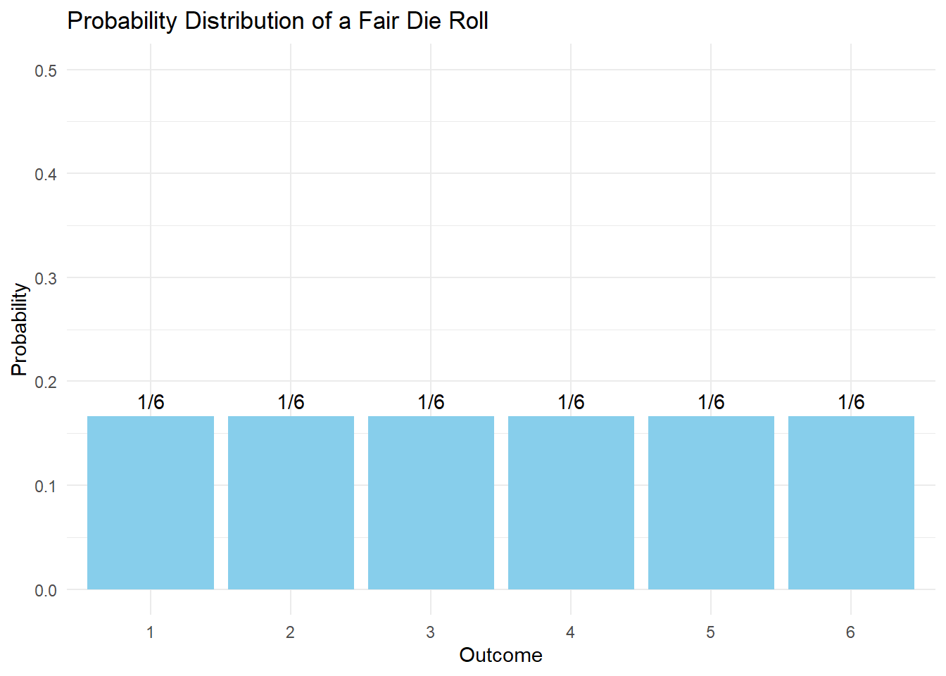
Bernoulli Distribution
The Bernoulli distribution is the simplest probability distribution, modeling a single “yes/no” trial.
Properties
- Only two possible outcomes: 0 (failure) or 1 (success)
- Controlled by single parameter p (probability of success)
- Mean: E(X) = p
- Variance: Var(X) = p(1-p)
Example: Biased Coin
# Visualization of Bernoulli distribution (p = 0.7)
bernoulli_data <- data.frame(
  outcome = c("Failure (0)", "Success (1)"),
  probability = c(0.3, 0.7)
)

ggplot(bernoulli_data, aes(x = outcome, y = probability)) +
  geom_bar(stat = "identity", fill = "lightgreen") +
  geom_text(aes(label = scales::percent(probability)), vjust = -0.5) +
  labs(title = "Bernoulli Distribution (p = 0.7)",
       x = "Outcome",
       y = "Probability") +
  theme_minimal() +
  ylim(0, 1)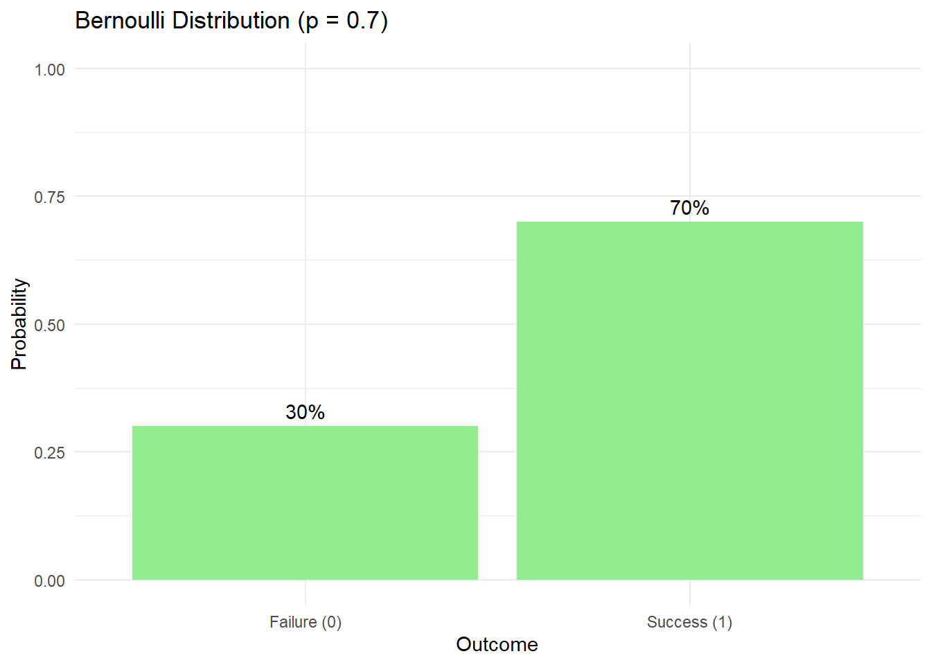
Binomial Distribution
The binomial distribution models the number of successes in n independent Bernoulli trials.
Properties
- Parameters: n (number of trials) and p (probability of success)
- Possible values: 0 to n successes
- Mean: E(X) = np
- Variance: Var(X) = np(1-p)
- Probability mass function: P(X = k) = \binom{n}{k} p^k (1-p)^{n-k}
Understanding the Formula
The binomial probability formula has three parts:
- \binom{n}{k} - Number of ways to get k successes in n trials
- p^k - Probability of k successes
- (1-p)^{n-k} - Probability of (n-k) failures
Visualizing Binomial Distributions
library(ggplot2)
# Function to calculate binomial probabilities
binomial_probs <- function(n, p) {
  k <- 0:n
  probs <- dbinom(k, n, p)
  data.frame(k = k, probability = probs)
}

# Create plots for different parameters
ggplot(binomial_probs(10, 0.5), aes(x = k, y = probability)) +
  geom_bar(stat = "identity", fill = "salmon") +
  labs(title = "Binomial(n=10, p=0.5)",
       x = "Number of Successes",
       y = "Probability") +
  theme_minimal()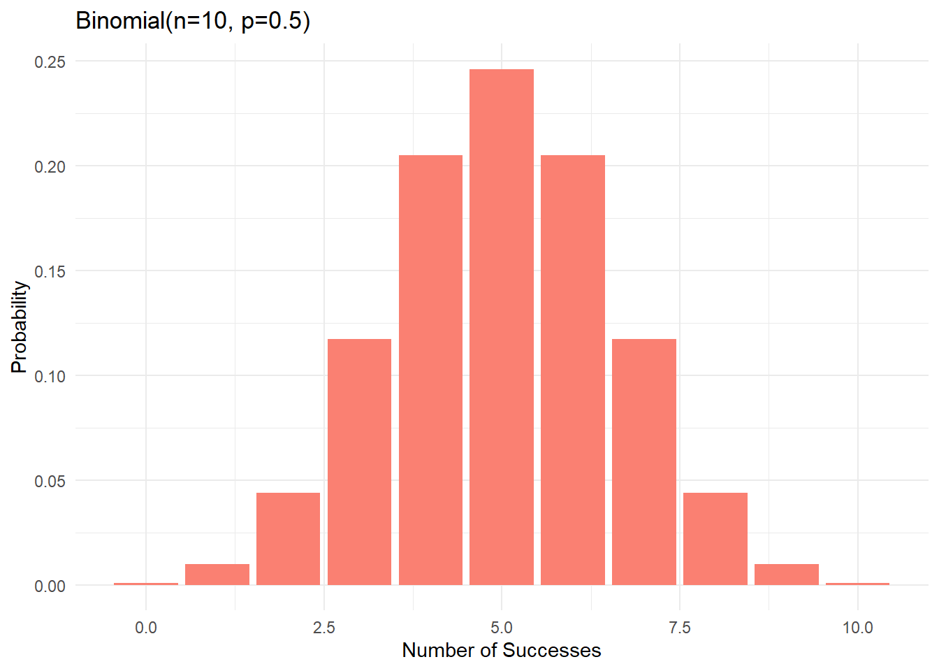
ggplot(binomial_probs(10, 0.2), aes(x = k, y = probability)) +
  geom_bar(stat = "identity", fill = "lightblue") +
  labs(title = "Binomial(n=10, p=0.2)",
       x = "Number of Successes",
       y = "Probability") +
  theme_minimal()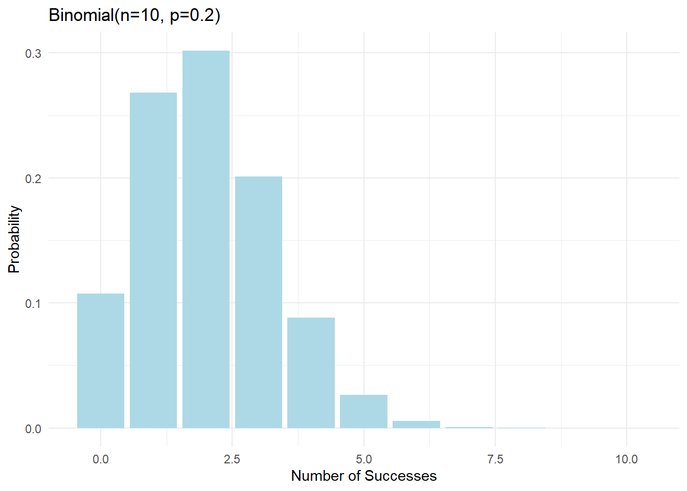
Effect of Parameters
The shape of the binomial distribution changes with n and p:
- Effect of n (number of trials):
- Larger n → more possible outcomes
- Larger n → distribution becomes more “bell-shaped”
- Effect of p (probability of success):
- p = 0.5 → symmetric distribution
- p < 0.5 → right-skewed distribution
- p > 0.5 → left-skewed distribution
Real-World Applications
- Quality Control
- n = number of items inspected
- p = probability of defect
- X = number of defective items found
- Clinical Trials
- n = number of patients
- p = probability of recovery
- X = number of patients who recover
Comparing the Distributions
Key differences between our three distributions:
- Uniform Distribution
- Equal probability for all outcomes
- Used when all outcomes are equally likely
- Example: rolling a fair die
- Bernoulli Distribution
- Special case of binomial with n = 1
- Only two possible outcomes
- Example: single coin flip
- Binomial Distribution
- Counts successes in multiple trials
- Combines multiple Bernoulli trials
- Example: number of heads in 10 coin flips
Interactive R Code for Exploration
# Function to compare distributions
compare_distributions <- function(n = 10, p = 0.5) {
  # Binomial probabilities
  x <- 0:n
  binom_probs <- dbinom(x, n, p)

  # Create data frame
  df <- data.frame(
    x = x,
    probability = binom_probs
  )

  # Create plot
  ggplot(df, aes(x = x, y = probability)) +
    geom_bar(stat = "identity", fill = "steelblue", alpha = 0.7) +
    geom_text(aes(label = round(probability, 3)), vjust = -0.5) +
    labs(title = sprintf("Binomial Distribution (n=%d, p=%.2f)", n, p),
         x = "Number of Successes",
         y = "Probability") +
    theme_minimal()
}

# Try different parameters
compare_distributions(n = 5, p = 0.5)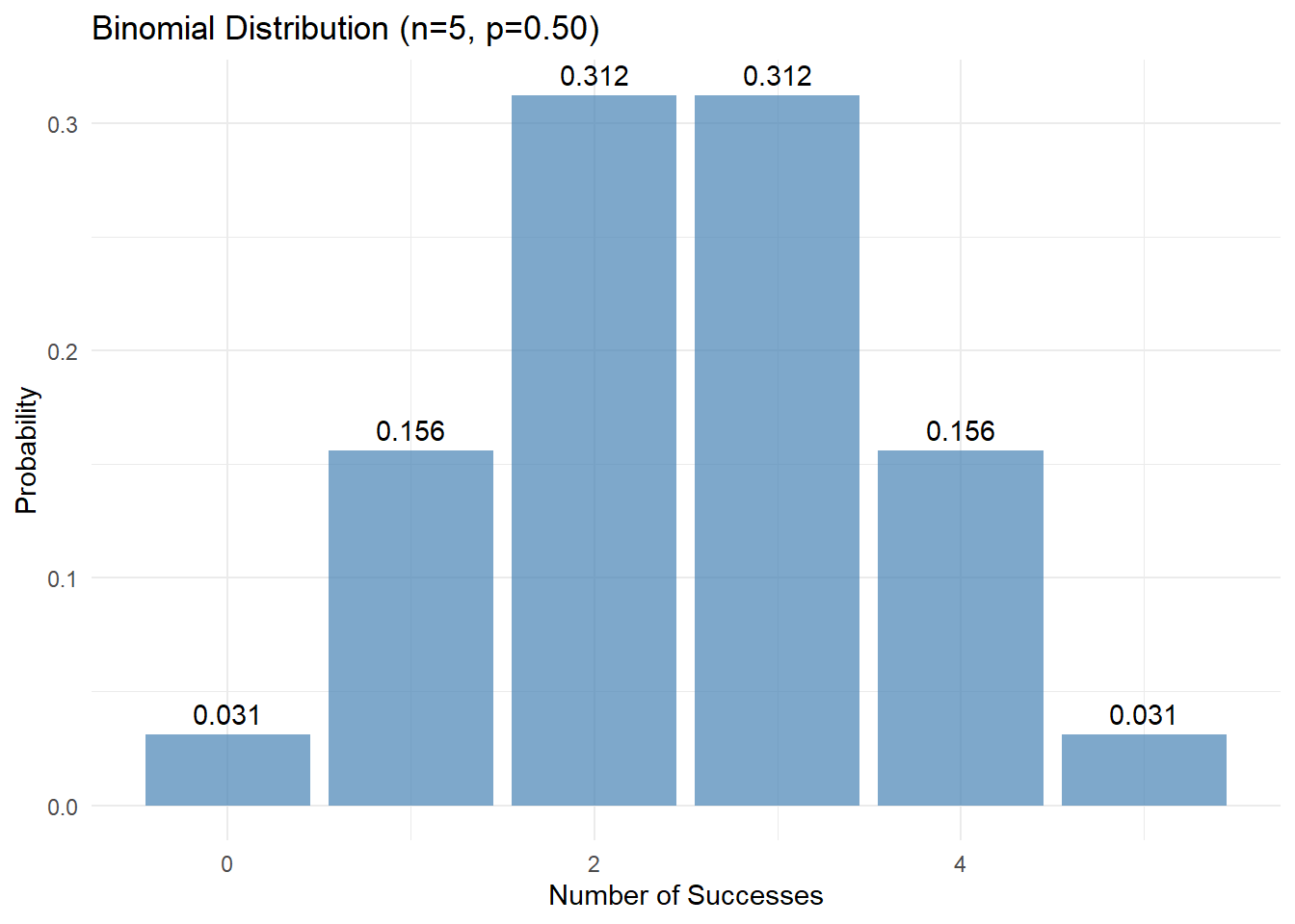
compare_distributions(n = 10, p = 0.3)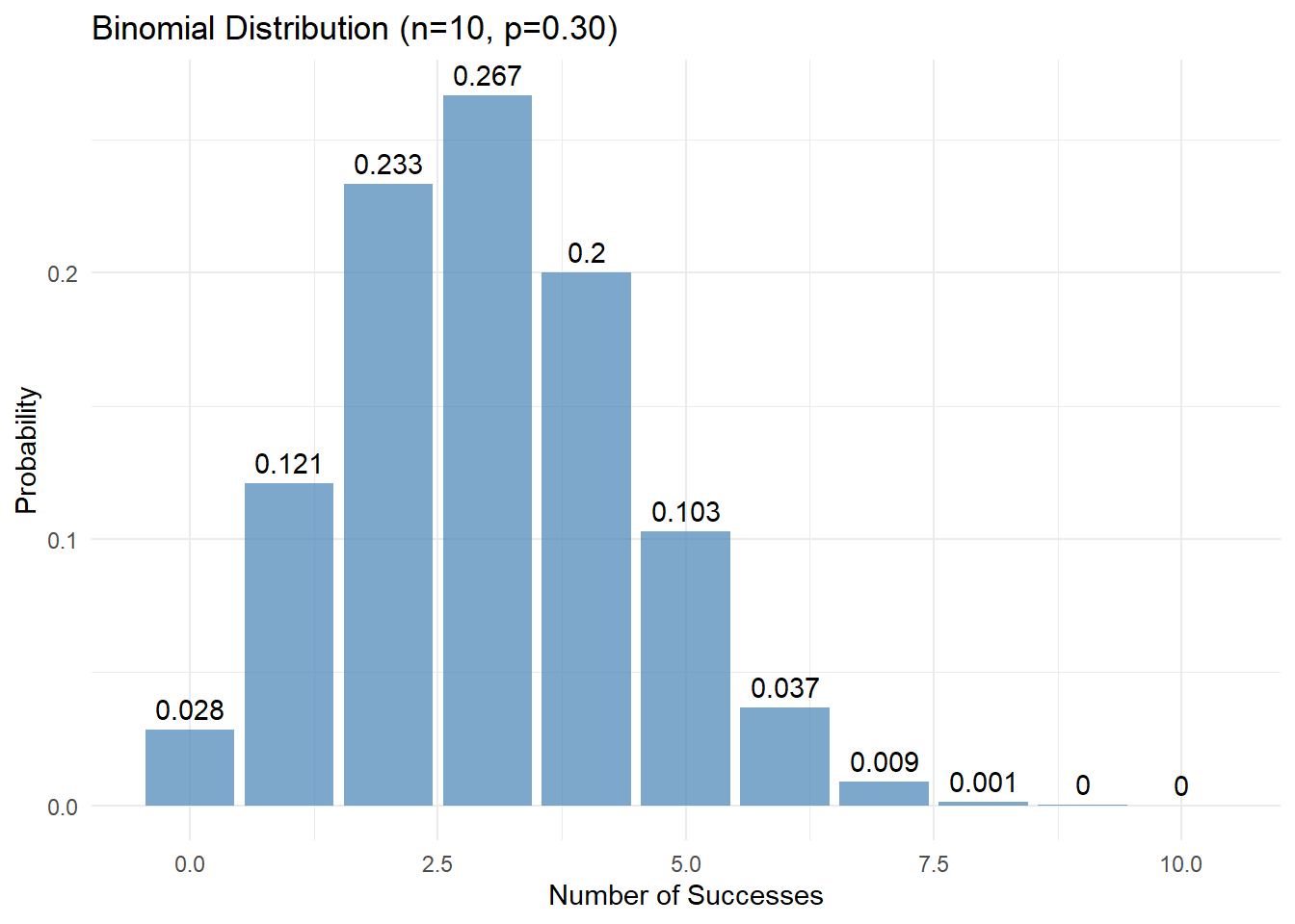
compare_distributions(n = 20, p = 0.7)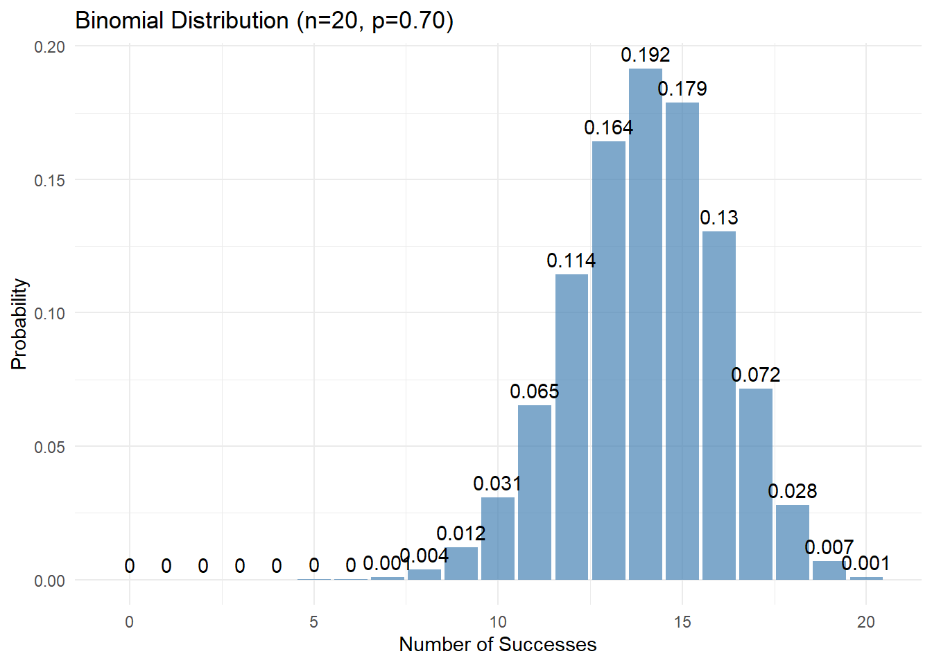
Applying Binomial Distribution: ESP Probability Analysis
Extrasensory perception (ESP), also known as a sixth sense, is a claimed ability to perceive information through mental means rather than the five physical senses.
Problem: A man claims to have extrasensory perception (ESP). To test this claim, a fair coin is flipped 10 times and the man is asked to predict each outcome in advance. He gets 7 out of 10 predictions correct. Calculate the probability of obtaining 7 or more correct predictions out of 10 trials by chance alone (assuming no ESP).
Remark: Under the null hypothesis of no ESP, the probability of each correct prediction is \frac{1}{2}.
Preliminary Concepts
Bernoulli Variable
A Bernoulli random variable represents a trial with exactly two possible outcomes: success (1) or failure (0). Each trial has probability p of success and 1-p of failure.
In our case, each coin flip prediction is a Bernoulli trial where success means a correct prediction.
Binomial Distribution
The binomial distribution extends the Bernoulli concept to model the sum of n independent Bernoulli trials. It describes the probability of obtaining exactly k successes in these n trials. The probability mass function is:
P(X = k) = \binom{n}{k}p^k(1-p)^{n-k}
where:
- n is the number of trials
- k is the number of successes
- p is the probability of success on each trial
- \binom{n}{k} is the binomial coefficient
Binomial Coefficient
The binomial coefficient \binom{n}{k} represents the number of ways to choose k items from n items, regardless of order. It is calculated as:
\binom{n}{k} = \frac{n!}{k!(n-k)!}
For example, \binom{10}{7} = \frac{10!}{7!(10-7)!} = \frac{10!}{7!3!} = 120
Problem Solution
Given: - n = 10 coin flips - p = \frac{1}{2} (probability of correct guess without ESP) - Need P(X \geq 7) = P(X = 7) + P(X = 8) + P(X = 9) + P(X = 10)
Step 1: Calculate P(X = 7) P(X = 7) = \binom{10}{7}(\frac{1}{2})^7(\frac{1}{2})^3 = 120 \cdot (\frac{1}{128}) \cdot (\frac{1}{8}) = 120 \cdot \frac{1}{1024} = \frac{120}{1024} \approx 0.117
Step 2: Calculate P(X = 8) P(X = 8) = \binom{10}{8}(\frac{1}{2})^8(\frac{1}{2})^2 = 45 \cdot (\frac{1}{256}) \cdot (\frac{1}{4}) = 45 \cdot \frac{1}{1024} = \frac{45}{1024} \approx 0.044
Step 3: Calculate P(X = 9) P(X = 9) = \binom{10}{9}(\frac{1}{2})^9(\frac{1}{2})^1 = 10 \cdot (\frac{1}{512}) \cdot (\frac{1}{2}) = 10 \cdot \frac{1}{1024} = \frac{10}{1024} \approx 0.010
Step 4: Calculate P(X = 10) P(X = 10) = \binom{10}{10}(\frac{1}{2})^{10}(\frac{1}{2})^0 = 1 \cdot (\frac{1}{1024}) \cdot 1 = \frac{1}{1024} \approx 0.001
Step 5: Sum all probabilities P(X \geq 7) = \frac{120 + 45 + 10 + 1}{1024} = \frac{176}{1024} \approx 0.172
Interpretation
There is approximately a 17.2% chance that someone without ESP would correctly guess 7 or more coin flips out of 10 by pure chance. This is a relatively high probability, suggesting that getting 7 out of 10 correct predictions is not strong evidence for ESP. Generally, we would want a much smaller probability (e.g., < 5% or < 1%) before considering the results statistically significant evidence for ESP.
Inductive Derivation of the Binomial Distribution Formula
Random Variable (X): A function that maps outcomes from a sample space to real numbers. In our case:
- X = number of successes in n trials
- X maps “Success” to 1 and “Failure” to 0 for each trial
- For n trials, X takes values in {0, 1, 2, …, n}
Probability Distribution: A function P(X = k) that assigns probabilities to each possible value k of the random variable X, where:
- P(X = k) ≥ 0 for all k
- \sum_{k=0}^n P(X = k) = 1
Let’s denote success as S and failure as F, with:
- Probability of success p = P(\text{Success}) = P(X = 1) for a single trial
- Probability of failure q = 1-p = P(\text{Failure}) = P(X = 0) for a single trial
1. One Trial
| Outcome | Ways | Probability |
|---|---|---|
| S | 1 | p |
| F | 1 | q |
Total outcomes: p + q = 1
2. Two Trials
| # Successes | Ways | Combinations | Probability |
|---|---|---|---|
| 2 | SS | 1 | p^2 |
| 1 | SF, FS | 2 | 2pq |
| 0 | FF | 1 | q^2 |
Notice: \binom{2}{k} gives us the number of ways (k = 0,1,2)
Total probability: p^2 + 2pq + q^2 = 1
3. Three Trials
| # Successes | Ways | Combinations | Probability |
|---|---|---|---|
| 3 | SSS | 1 | p^3 |
| 2 | SSF, SFS, FSS | 3 | 3p^2q |
| 1 | SFF, FSF, FFS | 3 | 3pq^2 |
| 0 | FFF | 1 | q^3 |
Here, \binom{3}{k} gives us the combinations (k = 0,1,2,3)
Total probability: p^3 + 3p^2q + 3pq^2 + q^3 = 1
Illustrating Coordinates for 3 Choose 2
For n = 3 and k = 2 successes, \binom{3}{2} = 3 gives us these success position coordinates:
| Success Positions | Sequence | Coordinate Interpretation |
|---|---|---|
| (1,2) | SSF | Successes in positions 1,2 |
| (2,3) | FSS | Successes in positions 2,3 |
| (1,3) | SFS | Successes in positions 1,3 |
This demonstrates why \binom{3}{2} = 3 - it counts all possible ways to choose 2 positions from 3 available positions.
4. Four Trials
| # Successes | Ways | Combinations | Coordinate Positions | Probability |
|---|---|---|---|---|
| 4 | SSSS | 1 | (1,2,3,4) | p^4 |
| 3 | SSSF, SSFS, SFSS, FSSS | 4 | (1,2,3), (1,2,4), (1,3,4), (2,3,4) | 4p^3q |
| 2 | SSFF, SFSF, SFFS, FSSF, FSFS, FFSS | 6 | (1,2), (1,3), (1,4), (2,3), (2,4), (3,4) | 6p^2q^2 |
| 1 | SFFF, FSFF, FFSF, FFFS | 4 | (1), (2), (3), (4) | 4pq^3 |
| 0 | FFFF | 1 | () | q^4 |
Note how \binom{4}{k} gives us the combinations:
- \binom{4}{4} = 1 (one way to choose all positions)
- \binom{4}{3} = 4 (four ways to choose 3 positions)
- \binom{4}{2} = 6 (six ways to choose 2 positions)
- \binom{4}{1} = 4 (four ways to choose 1 position)
- \binom{4}{0} = 1 (one way to choose no positions)
Total probability: p^4 + 4p^3q + 6p^2q^2 + 4pq^3 + q^4 = 1
Pattern Recognition and Generalization
For n trials:
- Each outcome has exactly n positions
- For k successes, we need k positions filled with S and (n-k) positions with F
- \binom{n}{k} gives us the number of ways to choose k positions for successes
- Each success contributes p, each failure contributes q
Therefore, for k successes in n trials:
- Ways = \binom{n}{k} (binomial coefficient)
- Probability of each way = p^k q^{n-k}
Binomial Distribution Formula
The probability of exactly k successes in n trials is:
P(X = k) = \binom{n}{k} p^k (1-p)^{n-k}
where:
- \binom{n}{k} counts the ways to arrange k successes in n positions
- p^k accounts for k successes
- (1-p)^{n-k} accounts for (n-k) failures
Coordinate System Interpretation
The binomial coefficient provides a systematic way to count all possible position combinations for successes. For example:
- In the 3-trial case with 2 successes (\binom{3}{2} = 3):
- Position 1 means success in first trial
- Position 2 means success in second trial
- Position 3 means success in third trial
- The coordinates (1,2), (2,3), (1,3) represent all possible ways to place 2 successes in 3 positions
- In the 4-trial case with 2 successes (\binom{4}{2} = 6):
- We get six distinct pairs of positions: (1,2), (1,3), (1,4), (2,3), (2,4), (3,4)
- Each pair represents a unique way to distribute 2 successes across 4 trials
- The remaining positions automatically become failures
This coordinate system demonstrates why the binomial coefficient is the correct counting tool: it systematically accounts for all possible ways to distribute k successes across n positions, where each position must be either a success or failure.
Understanding the Binomial Coefficient
The binomial coefficient \binom{n}{k} counts the number of ways to choose k items from n items, where order doesn’t matter. It relates to the multiplication rule through this key insight:
- First, count all possible ordered sequences (using multiplication rule)
- Then, divide by number of ways to arrange the k items (to remove order)
For example, to choose 2 items from 4:
- First position can be filled in 4 ways
- Second position can be filled in 3 ways
- Total ordered sequences = 4 × 3 = 12
- Number of ways to arrange 2 items = 2 × 1 = 2
- Therefore \binom{4}{2} = \frac{4 × 3}{2 × 1} = 6